Day 12 Repeated Measures III
12.2 Where we’re standing in this course
Considering the linear mixed model
\[\mathbf{y} \sim N(\mathbf{X}\boldsymbol{\beta}, \mathbf{V}),\] where:
- \(\mathbf{y}\) is the vector of the response,
- \(\mathbf{X}\) is the model matrix (often containing treatment allocation),
- \(\boldsymbol{\beta}\) is a vector containing the estimates for the effects of all variables in \(\mathbf{X}\),
- \(\mathbf{V}\) is the variance covariance matrix for \(\mathbf{y}\).
The marginal distribution of \(\mathbf{y}\) for a normal distribution can also be written as \[\mathbf{y} \sim MVN(\mathbf{X}\boldsymbol{\beta}, \mathbf{ZGZ}'+\mathbf{R}).\]
The variance-covariance matrices below represent the variance/covariance of all \(y\)s.

Figure 12.1: Illustrative example of the variance-covariance matrix.
We consider messy data the different dependence patterns in \(\mathbf{G}\) and/or \(\mathbf{R}\).
Note that, for all mixed models we have been handling so far, \[\mathbf{G} = \sigma^2_u\mathbf{I} = \begin{bmatrix} \sigma^2_u & 0 & 0 & & 0\\ 0 & \sigma^2_u & 0 & & 0\\ 0 & 0 & \sigma^2_u & & 0\\ & & & \ddots & \vdots \\ 0 & 0 & 0 & \dots & \sigma^2_u\\ \end{bmatrix},\] which, will result in some variation of the matrix above.
12.3 Repeated measures

Figure 12.2: Schematic description of a field experiment with repeated measures
12.4 Correlation - G side (conditional) and R side (marginal)
- Typically,
REPEATED(in SAS’sMIXEDprocedure) is equivalent to R-side (marginal) covariance inGLIMMIX. - Look at marginal variance-covariance matrix on the board.
- What happens if we model G-side covariance?
Implications on inference
- Similar CI for marginal means (lsmeans)
- Confidence intervals estimated with different DF approximations
- May see some discrepancy in test statistics.
12.5 Repeated measures in GLMMs
Recall distributions of non-Gaussian GLMMs:
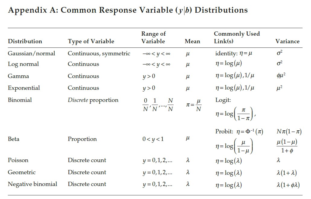
Figure 12.3: Common variable distributions. Page 60 in Stroup et al. (2024)
12.6 Appendix A: Common Response Variable (\(y | b\)) Distributions
Below is a table of commonly used distributions, their properties, and related probability density functions (PDFs).
| Distribution | Range of Variable | Mean | Commonly Used Link(s) | Variance | |
|---|---|---|---|---|---|
| Gaussian/normal | \(-\infty < y < \infty\) | \(\mu\) | \(\eta = \mu\) | \(\sigma^2\) | \[f(y) = \frac{1}{\sqrt{2\pi \sigma^2}} e^{-\frac{(y-\mu)^2}{2\sigma^2}}\] |
| Log normal | \(-\infty < y < \infty\) | \(\mu\) | \(\eta = \log(\mu)\) | \(\sigma^2\) | \[f(y) = \frac{1}{y\sigma\sqrt{2\pi}} e^{-\frac{(\log y - \mu)^2}{2\sigma^2}}\] |
| Gamma | \(y > 0\) | \(\mu\) | \(\eta = \log(\mu), \frac{1}{\mu}\) | \(\phi \mu^2\) | \[f(y) = \frac{y^{\frac{\mu}{\phi} - 1} e^{-\frac{y}{\phi}}}{\phi^{\mu} \Gamma(\mu)}\] |
| Exponential | \(y > 0\) | \(\mu\) | \(\eta = \log(\mu), \frac{1}{\mu}\) | \(\mu^2\) | \[f(y) = \frac{1}{\mu} e^{-\frac{y}{\mu}}\] |
| Binomial | 0, \(\frac{1}{N}, \dots, \frac{N}{N}\) | \(\pi = \frac{\mu}{N}\) | Logit: \(\eta = \log\left(\frac{\pi}{1-\pi}\right)\) | \(N\pi(1-\pi)\) | \[f(y) = \binom{N}{y} \pi^y (1-\pi)^{N-y}\] |
| Beta | 0 < \(y < 1\) | \(\mu\) | \(\eta = \log\left(\frac{\mu}{1-\mu}\right)\) | \(\frac{\mu(1-\mu)}{1+\phi}\) | \[f(y) = \frac{y^{\alpha-1}(1-y)^{\beta-1}}{B(\alpha, \beta)}\] |
| Poisson | \(y = 0, 1, 2, \dots\) | \(\lambda\) | \(\eta = \log(\lambda)\) | \(\lambda\) | \[f(y) = \frac{\lambda^y e^{-\lambda}}{y!}\] |
| Geometric | \(y = 0, 1, 2, \dots\) | \(\lambda\) | \(\eta = \log(\lambda)\) | \(\lambda(1+\lambda)\) | \[f(y) = (1-\lambda)^y \lambda\] |
| Negative binomial | \(y = 0, 1, 2, \dots\) | \(\lambda\) | \(\eta = \log(\lambda)\) | \(\lambda(1+\phi\lambda)\) | \[f(y) = \binom{y + r - 1}{y} \lambda^r (1-\lambda)^y\] |
If we describe a non-Gaussian GLMM with
\[{y}|\boldsymbol{u} \sim P({\mu}, \phi),\] where \(y\) is the response, \(\boldsymbol{u}\) are the random effects, \(\mu\) is the mean, and \(\phi\) is the dispersion, we know that \(\mu\) and \(\phi\) may not be independent.
- G-side ~ ‘true GLMM’
- R-side: quasi-likelihood models
- Marginal models often lead to less powerful tests.
- Several discussions:
- Philosophical, Power, and more Lee and Nelder (2004)
- Many unknowns for the software implementation of non-Gaussian GLMMs Stroup and Claassen (2020)