Day 13 Modeling designed experiments in the presence of spatial variability

October 8th

13.1 Announcements

• Zoom classes on 10/13 and 10/15.
• Assignment 4 due today midnight.

13.2 Spatial variability

• Most commonly found in field experiments.
• Whiteboard: going from the normal iid model to a spatial dependence model.

13.2.1 Spatial patterns

Consider the model \[\mathbf{y} \sim N(\boldsymbol{\mu}, \boldsymbol{\Sigma}),\] where \(\boldsymbol{\Sigma}\) is the variance-covariance model. In the presence of spatial patterns, there are parametric and non-parametric tools to account for spatial dependence.

Sometimes, we can clearly define the shape of the spatial dependence pattern. For example:

Matérn covariance function

\[C(d; \sigma^2, \phi, \kappa) = \sigma^2 \frac{(h/\phi)^\kappa K_\kappa (h/\phi)}{2^{\kappa-1} \Gamma(\kappa)}\]

Gaussian covariance function

\[C(d; \sigma^2, \phi) = \sigma^2 \exp \left\{ - \frac{d^2}{2\phi^2} \right\} \]

Exponential covariance function

\[C(d; \sigma^2, \phi, \kappa) = \sigma^2 \exp\{-(d/\phi)^\kappa\}\]

13.2.2 Applied example

Yield data from an advanced Nebraska Intrastate Nursery (NIN) breeding trial conducted at Alliance, Nebraska, in 1988/89.

library(tidyverse)
library(agridat)
library(ggpubr)
data <- drop_na(stroup.nin)

data %>% 
  ggplot(aes(col, row))+
  geom_tile(aes(fill = rep), color = "black")+
  theme_pubr()+
  labs(fill = "Block")+
  theme(axis.line = element_blank())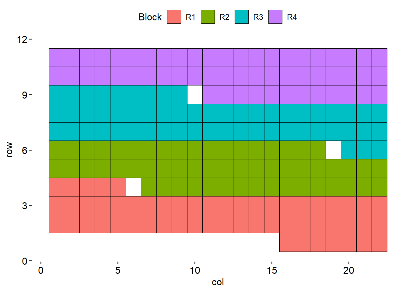

The statistical model:

\[y_{ij}\sim N(\mu_{ij}, \sigma^2), \\ \mu_{ij} = \eta_{ij} = \eta_0 + G_i + b_j, \\ b_j \sim N(0, \sigma^2_b).\]

Assumptions:

• iid, normal residuals

library(lme4)
m <- lmer(yield ~ gen + (1|rep), data = stroup.nin)
data$res <- resid(m)

data %>% 
  ggplot(aes(col, row))+
  geom_tile(aes(fill = res), color = "black")+
  theme_pubr()+
  scico::scale_fill_scico()+
  theme(axis.line = element_blank())+
  labs(fill = expression(Residual~(bu~ac^{-1})))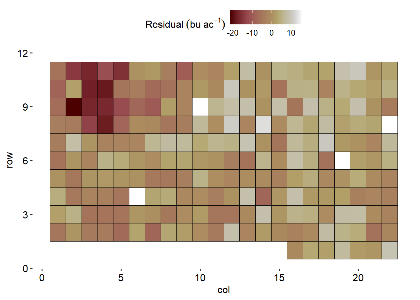

as.data.frame(emmeans(m, ~ gen)) %>% 
  arrange(-emmean) %>% 
  head()

##  gen        emmean       SE    df lower.CL upper.CL
##  NE86503   32.6500 3.855689 66.69 24.95335 40.34665
##  NE87619   31.2625 3.855689 66.69 23.56585 38.95915
##  NE86501   30.9375 3.855689 66.69 23.24085 38.63415
##  Redland   30.5000 3.855689 66.69 22.80335 38.19665
##  Centurk78 30.3000 3.855689 66.69 22.60335 37.99665
##  NE83498   30.1250 3.855689 66.69 22.42835 37.82165
## 
## Degrees-of-freedom method: kenward-roger 
## Confidence level used: 0.95

library(glmmTMB)

data$coordinate <- numFactor(data$col, data$row)
data$group <- factor(1) 

m_spatial <- glmmTMB(yield ~ gen + (1|rep) + mat(coordinate + 0 | group), data = data)

data$resid_spatial <- resid(m_spatial)

data %>% 
  ggplot(aes(col, row))+
  geom_tile(aes(fill = resid_spatial), color = "black")+
  theme_pubr()+
  scico::scale_fill_scico()+
  theme(axis.line = element_blank())+
  labs(fill = expression(Residual~(bu~ac^{-1})))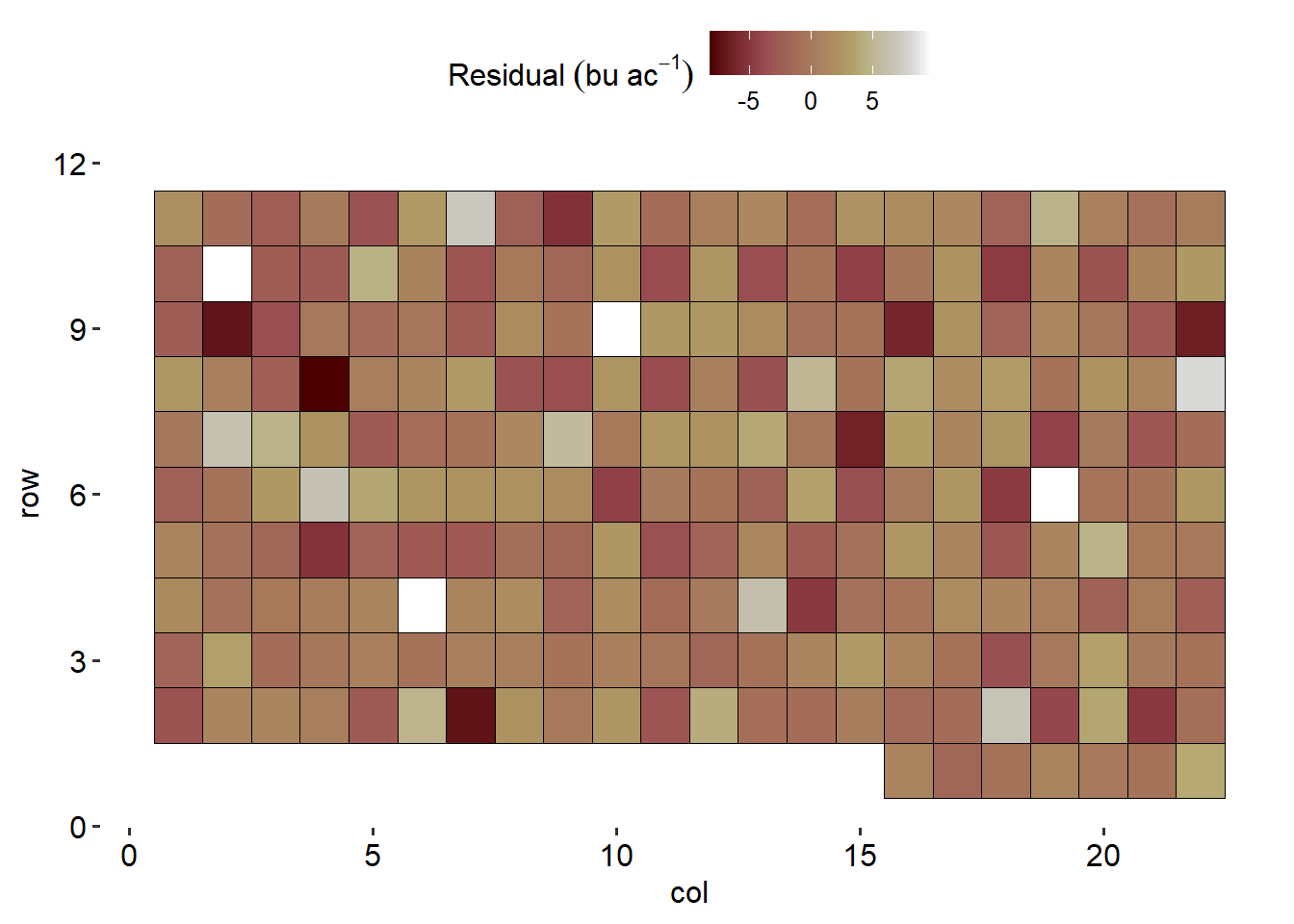

as.data.frame(emmeans(m_spatial, ~ gen)) %>% 
  arrange(-emmean) %>% 
  head()

##  gen        emmean       SE  df asymp.LCL asymp.UCL
##  Buckskin 33.37166 3.399255 Inf  26.70925  40.03408
##  NE85556  29.35020 3.395673 Inf  22.69480  36.00560
##  NE87619  29.09390 3.397032 Inf  22.43584  35.75196
##  NE83498  28.90073 3.405042 Inf  22.22697  35.57449
##  Redland  28.63517 3.393941 Inf  21.98317  35.28717
##  NE86503  27.51328 3.451773 Inf  20.74792  34.27863
## 
## Confidence level used: 0.95