Day 5 Linear mixed models
September 10th
5.1 Announcements
- Assignment 2 is due today!
5.2 Linear mixed models
Mixed models come in handy when the (in)famous independence assumption cannot be taken for granted, especially if we know the dependence patterns in the data. We typically know the dependence patterns in the data when running an experiment. For example, the fungicide-barley experiment. Let’s re-do the statistical model and ANOVA shell:
A reasonable model could be
\[y_{ijk}|b_k, u_{i(k)} \sim N(\mu_{ijk}, \sigma_e^2),\]
\[\mu_{ijk} = \eta_{ijk},\] \[\eta_{ijk} = \eta_0 + F_i +G_j + (FG)_{ij}+b_k+ u_{i(k)},\]
where:
- \(y_{ijk}\) is the observed yield for the \(i\)th fungicide treatment, \(j\)th genotype treatment, and \(k\)th repetition,
- \(\mu_{ijk}\) is the expected value for the \(i\)th fungicide treatment, \(j\)th genotype treatment, and \(k\)th repetition,
- \(\sigma^2\) is the residual variance,
- \(\eta_{ijk}\), the linear predictor is equivalent to the expected value because the link function is the identity function,
- \(\eta_0\) is the overall mean of the linear predictor,
- \(F_i\) is the effect of the \(i\)th fungicide treatment,
- \(G_j\) is the effect of the \(j\)th genotype treatment,
- \((FG)_{ij}\) is the interaction for the \(i\)th fungicide treatment and \(j\)th genotype treatment,
- \(b_k\) is the effect of the \(k\)th block, \(b_k \sim N(0, \sigma^2_b)\)
- \(u_{i(k)}\) is the effect of the whole plot corresponding to the \(i\)th fungicide treatment in the \(k\)th block, \(u_{i(k)} \sim N(0, \sigma^2_u)\).
A reasonable ANOVA shell could be:
| Source | df |
|---|---|
| - | - |
| Fungicide | f-1 = 1 |
| - | - |
| Genotype | g-1 = 69 |
| Fung x Gen | (f-1)(g-1) = 69 |
| Error | N-fg = 420 |
| Total | N-1 |
| Source | df |
|---|---|
| Block | b-1 |
| Fungicide | f-1 |
| Fungicide(Block) | (b-1)(f-1) |
| Genotype | g-1 |
| Fung x Gen | (f-1)(g-1) |
| Gen(Block x Fung) | f(b-1)(g-1) |
| Total | N-1 |
| Source | df |
|---|---|
| Block | 3 |
| Fungicide | 1 |
| Fungicide(Block) | 3 |
| Genotype | 69 |
| Fung x Gen | 69 |
| Gen(Block x Fung) | 414 |
| Total | 559 |
Notice that the 420 degrees of freedom (aka independent observations) from the CRD ANOVA are now spread across different levels, connected to different variance components: blocks, whole plots, and random error. This means that there is a different number of independent observations for Fungicide compared to Genotype. The variance components will affect the inference distinctly:
- Standard errors for comparisons at the whole plot: \(se(\mu_{i\cdot}-\mu_{i'\cdot}) = \sqrt{\frac{2(\sigma^2_e + g\sigma^2_u)}{gb}}\)
- Standard errors for comparisons at the split plot: \(se(\mu_{\cdot j}-\mu_{\cdot j'}) = \sqrt{\frac{2 \sigma^2_e }{fb}}\)
Let’s apply that model:
library(lme4)

# load the data
url <- "https://raw.githubusercontent.com/stat870/fall2025/refs/heads/main/data/fung_barley_sp.csv"
fung_sp <- read.csv(url)

fung_sp %>%
  ggplot(aes(bed, row))+
  coord_fixed()+
  theme_minimal()+
  geom_tile(aes(fill = fung))+
  geom_tile(aes(), color = "black", fill = NA)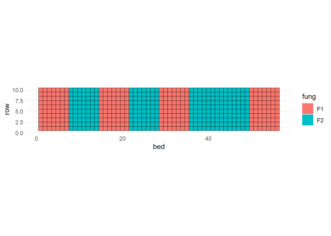
# fit the model
m <- lmer(yield ~ fung*gen + (1|block/fung), data = fung_sp)

# anova
car::Anova(m, type = 2, test.statistic = "F")
## Analysis of Deviance Table (Type II Wald F tests with Kenward-Roger df)
##
## Response: yield
## F Df Df.res Pr(>F)
## fung 40.2718 1 3 0.007915 **
## gen 7.2008 69 414 < 2.2e-16 ***
## fung:gen 0.9331 69 414 0.629010
## ---
## Signif. codes: 0 '***' 0.001 '**' 0.01 '*' 0.05 '.' 0.1 ' ' 15.2.1 Why do we call these multi-level models?
The data are clustered in groups that were generated under similar conditions.
- What are those groups in the barley example?
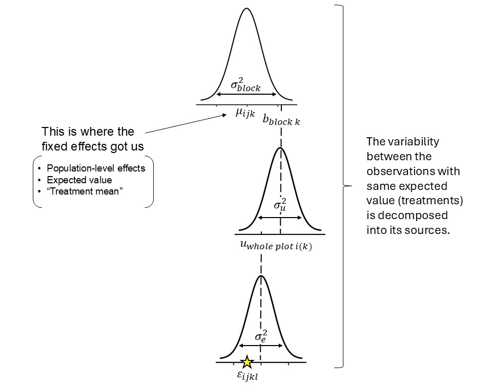
Figure 5.1: Intuitive visualization of a split-plot design model as a hierarchical (multilevel) model.
5.2.2 Degrees of freedom in a mixed model
Degrees of freedom for means are not that easy and straightforward to compute under mixed models anymore. There are approximate methods to calculate the degrees of freedom, like Satterthwaite or Kenward-Roger.
##  fung gen emmean    SE   df lower.CL upper.CL
##  F1   G01   5.24 0.174 31.4     4.88     5.59
##  F2   G01   4.58 0.174 31.4     4.23     4.94
##  F1   G02   5.38 0.174 31.4     5.02     5.73
##  F2   G02   4.75 0.174 31.4     4.39     5.11
##  F1   G03   6.53 0.174 31.4     6.18     6.89
##  F2   G03   5.62 0.174 31.4     5.26     5.97
##
## Degrees-of-freedom method: kenward-roger
## Confidence level used: 0.95
However, computing the degrees of freedom for the comparisons is much more straightforward (esp. because this a balanced design).
- Take a look at the ANOVA table, and the experimental units.
sigma2_e <- sigma(m)^2
sigma2_wp <- as.data.frame(VarCorr(m))[1,]$vcov
sigma2_b <- as.data.frame(VarCorr(m))[2,]$vcov
levels_wp <- dplyr::n_distinct(fung_sp$fung)
levels_sp <- dplyr::n_distinct(fung_sp$gen)
reps <- dplyr::n_distinct(fung_sp$block)
Differences between levels of the factor at the whole plot – \(se(\mu_{i\cdot}-\mu_{i'\cdot}) = \sqrt{\frac{2(\sigma^2_e + g\sigma^2_u)}{gb}}\).
# get the s.e. for comparisons between fungicide treatments by hand
sqrt( 2*(sigma2_e + levels_sp*sigma2_wp) / (levels_sp*reps))
## [1] 0.086331## NOTE: Results may be misleading due to involvement in interactions## contrast estimate SE df t.ratio p.value
## c(1, -1) 0.548 0.0863 3 6.346 0.0079
##
## Results are averaged over the levels of: gen
## Degrees-of-freedom method: kenward-rogerDifferences between levels of the factor at the split plot – \(se(\mu_{\cdot j}-\mu_{\cdot j'}) = \sqrt{\frac{2 \sigma^2_e }{fb}}\).
# get the s.e. for comparisons between genotype treatments by hand
sqrt( 2*(sigma2_e ) / (levels_wp*reps))
## [1] 0.1405927## NOTE: Results may be misleading due to involvement in interactions## contrast
## c(1, -1, 0, 0, 0, 0, 0, 0, 0, 0, 0, 0, 0, 0, 0, 0, 0, 0, 0, 0,
## estimate SE df t.ratio p.value
## -0.152 0.141 414 -1.085 0.2787
##
## Results are averaged over the levels of: fung
## Degrees-of-freedom method: kenward-roger