Day 27 Bayesian analysis of data generated by designed experiments
27.1 Announcements
- Project deadlines:
- December 12th: give your presentation by this date (it can be earlier than this also). You will need to schedule a 30min meeting with me.
- December 19th: submit your final project and tutorial on canvas, including both your classmate’s and my feedback.
27.2 Applied example
Suppose we designed an experiment with the rationale outlined above. What if the model doesn’t converge?
- About dropping effects from the model
- Bayesian solutions
dat <- readxl::read_xlsx("../../data_confid/Behavior_Counts.xlsx")

# viz
dat |>
  ggplot(aes(timepoint, behavior_count))+
  geom_line(aes(group = calfID,
                color = breed))+
  geom_point(aes(group = breed,
                 fill = breed),
             shape =21, size= 2.5)+
  facet_wrap(~trt)+
  scico::scale_fill_scico_d()+
  scico::scale_color_scico_d()+
  theme_pubclean()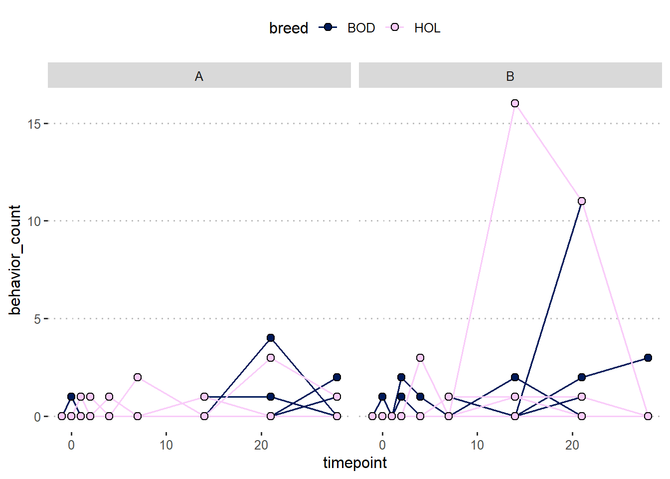
m2 <- glmmTMB(behavior_count ~ timepoint * trt * breed +
                toep(timepoint + 0 | calfID),
              ziformula = ~1,
              family = poisson(link = "log"),
              data = dat |> mutate(timepoint_f=as.factor(timepoint)))
What to do?

Figure 27.1: That’s all!