Day 24 Model selection
24.1 Announcements
- Project deadlines:
- December 5th: return your peer review to your classmate(s).
- December 12th: give your presentation by this date (it can be earlier than this also). You will need to schedule a 30min meeting with me.
- December 19th: submit your final project and tutorial on canvas, including both your classmate’s and my feedback.
24.2 Model selection
- Review: building a statistical model
- Models for data generated by designed experiments
- Convergence issues in models for data generated by designed experiments
- Loss functions
What is a model? Using word association, an obvious matchto model is airplane. We are all familiar with model airplanes,which come in a variety of shapes, sizes, and prices. Theessential feature of a model airplane is that it is simpler andcosts less but nonetheless captures some relevant features of areal airplane. Scientific and statistical models are simplifi-cations of the world around us, which is why we use the wordmodel in the same way as for model airplanes. Like modelairplanes, scientific models can come in a variety of forms andsizes, ranging from a simple average of data, to global climatemodels. Because models have variety, it is natural to considerwhen models are good or useful (Box 1976, Box and Draper1987:74, 424), which naturally leads to considering when 1model is better than another, and indeed searching for thebest model, or combination of models. The search, then, is animportant part of overall inference, i.e., how that searchaffects the global uncertainty, risk, and the probability ofmaking errors.
From Ver Hoef and Boveng (2015)
Model selection in other contexts
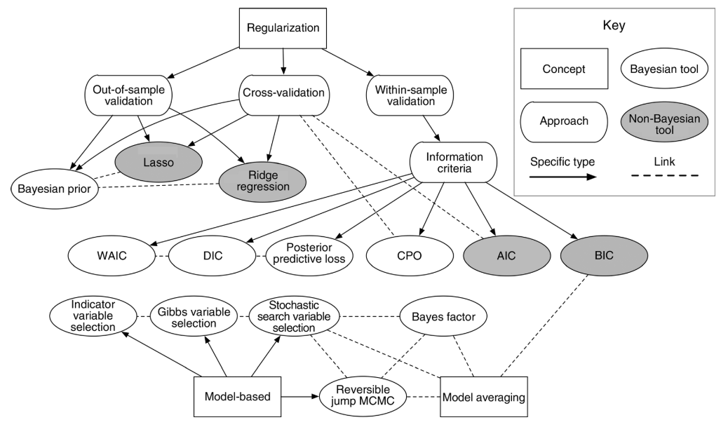
Figure 24.1: Figure 2 in Hooten and Hobbs (2015)
24.2.1 The coefficient of determination R2
- Usually interpreted as the proportion of the variation in \(y\) that is explained with the variation in \(x\).
- Used as a metric for predictive ability and model fit.
- Can increase when adding more predictors.
The R2 of a given model (and observed data) is calculated as \[R^2 = \frac{MSS}{TSS}= 1 - \frac{RSS}{TSS} = 1- \frac{MSE}{MST},\] where \(RSS\) is the residual sum of squares and \(TSS\) is the total sum o squares, and \(MSE\) is the mean squared error and \(MST\) is the mean squared of the data (i.e., \(y\) versus \(\bar{y}\).
24.2.2 Adjusted R2
The adjusted R2 also penalizes the addition of extra parameters
\[R^2_{adj} = R^2 - (1 - R^2) \frac{p-1}{n-p},\]
where \(R^2\) is the one defined above, \(p\) is the number of parameters and \(n\) is the total number of observations.
24.2.3 Some issues with R2
- Bootstrapped R2
- Anscombe’s quartet
- Out-of-Sample R2: Estimation and Inference
24.2.4 Akaike Information Criterion (AIC)
- Used as a metric for predictive ability and model fit.
- Lower value is better.
- Values are always compared to other models (i.e., there are no general rules about reasonable AIC values).
The AIC of a given model \(M\) and observed data \(\mathbf{y}\) is calculated as
\[AIC_M = 2p - 2\log(\hat{L}),\]
\(p\) is the number of parameters estimated in the model and \(\hat{L}\) is the maximized value of the likelihood function for the model (i.e., \(\hat{L}=p(\mathbf{y}|\hat{\boldsymbol\beta}, M)\)).
24.2.5 Bayesian Information Criterion (BIC)
The BIC of a given model (and observed data) is a variant of AIC and is calculated as
\[BIC = p\log(n) - 2\log(\hat{L}),\]
where \(p\) is the number of parameters estimated in the model, \(n\) is the number of observations, and \(\hat{L}\) is the maximized value of the likelihood function for the model (i.e., \(\hat{L}=p(\mathbf{y}|\hat{\boldsymbol\beta}, M)\)).
24.3 Regularization
- These methods are sometimes a useful alternative for scenarios where the predictors present collinearity.
- regularization, shrinkage, penalization.
Refresh: Ordinary Least Squares Regression
\[\hat{\beta}_{OLS}=(\mathbf{X}^\top\mathbf{X})^{-1}\mathbf{X}^\top\mathbf{y}\]
24.3.1 Ridge Regression
- Solve \(\underset{\beta}{\text{argmin}} = (\mathbf{y}-\mathbf{X}\beta)^\top(\mathbf{y}-\mathbf{X}\beta)+\lambda(\beta^\top \beta - c)\).
- \(\hat{\beta}_{\text{Ridge}}=(\mathbf{X}^\top\mathbf{X}+\lambda\mathbf{I})^{-1}\mathbf{X}^\top\mathbf{y}\).
- \(\hat{\beta}_{\text{Ridge}}\) for \(\lambda = 0\).
- As the ridge parameter \(\lambda\) increases, the estimates can become close to zero.
- Useful for cases with collinearity and unstable \(\hat{\beta}_{OLS}\).
- Pick the smallest value of \(\lambda\) that produces stable estimates of \(\beta\).
- There are also automatic selections of \(\lambda\).
24.3.2 Lasso Regression
- Lasso = Least absolute shrinkage and selection operator
- Solve \(\underset{\beta_0, \beta }{\text{argmin}} = \left\{ \sum_{i=1}^{N}(y_i - \beta_0 - x_i^T \beta)^2 \right\} \text{subject to} \sum_{j=1}^{p}|\beta_j| \leq t\).
- \(\hat{\beta}\) does not have a closed form solution.
- As penalization increases, the \(\beta\) estimates can become zero.
- Not great for cases with collinearity. Elastic net is a better alternative.
- Problems with high-dimensional data (e.g., genetics data). Elastic net is a better alternative.
24.3.3 Elastic Net Regression
- Combines the L1 (Lasso) and L2 (Ridge) regularization penalties.
- \(\hat{\beta} \equiv \underset{\beta}{\text{argmin}}(||y-\mathbf{X}\beta||^2 +\lambda_2||\beta||^2 +\lambda_1||\beta||_1)\), where \(||\beta||_1 = \sum_{j=1}^{p}|\beta_j|\).
- Ridge and Lasso are special cases of Elastic Net.
24.6 References
- Out of sample R2 Hawinkel et al. (2024)
- Model selection Hooten and Hobbs (2015)
- Multimodel inference Burnham and Anderson (2004)
- Iterating over a single model is a viable alternative to multimodel inference ver Hoef and Boveng (2015)