Day 16 Accounting for spatial effects
16.3 Non-parametric tools
- Minimize/relax assumptions
- No free lunches!
- Interpretability
- bias-variance tradeoff
16.3.1 Splines
- Splines are special cases of non-parametric tools.
- Introduced in the sixties (Schoenberg, 1964)
- They provide a flexible tool to model the variability in the data, where the functional (~ “the shape”) is unknown
Polynomials:
- good for local approximation
- bad for global approximation
16.4 B-splines
We can generally describe smoothing splines as the sum of many basis functions: \[f(x) = \sum_{i=1}^k B_i^m(x) \beta_i \]
Expanded equation: \[f(x) = \beta_0 + \beta_1 x +\beta_2 x^2 +\dots + \beta_p x^p + \left\{ b_1(x - \kappa_1)^p_{+} + b_2(x - \kappa_2)^p_{+} + \dots + b_K(x - \kappa_K)^p_{+} \right\},\] where:
- \(\kappa_1, \kappa_2, \dots, \kappa_K\) are the knots,
- \(b_1, b_2, \dots, b_K\) are the spline coefficients.
Using matrix notation: \[f(X_i) = \beta_0 + X_i \beta_1 + X^2_i \beta_2 + \dots + X_i^p \beta_p \\+ b_1(X_i - \kappa_1)^p_+ + b_2(X_i - \kappa_2)^p_+ + \dots + b_K(X_i - \kappa_K)^p_+ \\ = \mathbf{X}_i^T \boldsymbol{\beta}_X + \mathbf{B}^T(X_i)\mathbf{b},\] minimize: \[\sum_{i=1}^n \left\{ Y_i - (\mathbf{X}_i^T \boldsymbol{\beta}_X + \mathbf{B}^T(X_i)\mathbf{b}) \right\}^2 + \lambda \mathbf{b}^T\mathbf{Db},\] where \(\lambda \mathbf{b}^T\mathbf{Db}\) prevents overfitting:
- \(\mathbf{D}\) positive semidefinite.
- \(\lambda\) controls penalization and is very important.
Then, for a straight line:
\[f(x) = \beta_0 + \beta_1 x + \left\{ b_1(x - \kappa_1)_{+} + b_2(x - \kappa_2)_{+} + \dots + b_K(x - \kappa_K)_{+} \right\},\] where:
- \(\kappa_1, \kappa_2, \dots, \kappa_K\) are the knots,
- \(b_1, b_2, \dots, b_K\) are the spline coefficients.
16.4.1 Illustrating splines
Let’s start with a simple piecewise linear regression. Take the following data example:
set.seed(2)
df <- data.frame(x = seq(1, 50, by = .3)) %>%
  mutate(y = 10  + 4*cos(.4*x) + rnorm(n(), 0, 2))

df %>%
  ggplot(aes(x, y))+
  geom_point(alpha= .2)+
  theme_pubclean()+
  labs(x = "Some predictor",
       y = "Some response")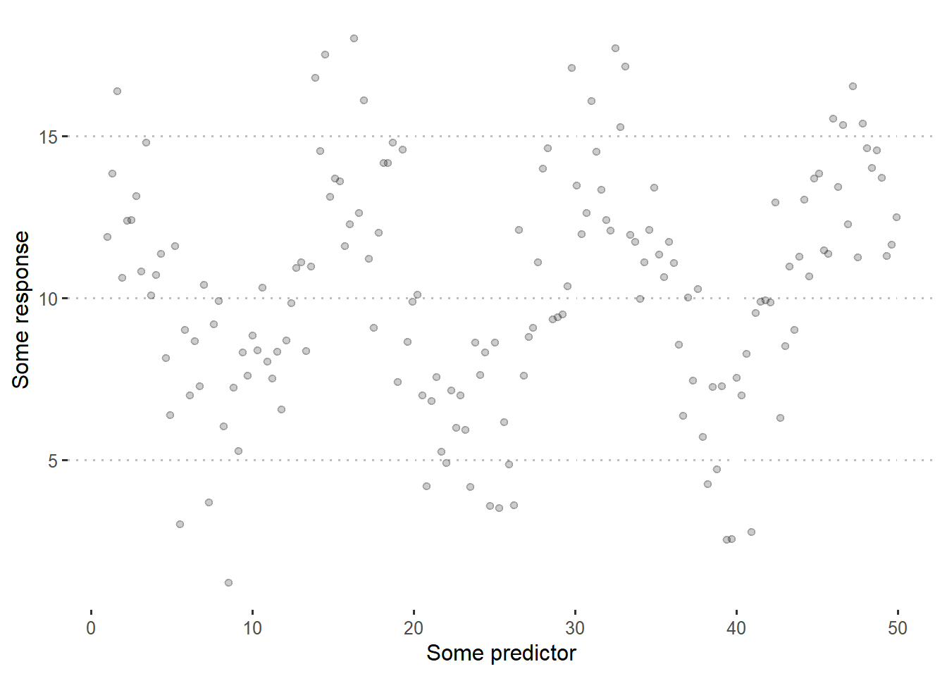
Let’s start with \[f(x) = \sum_{i=1}^k B_i^m(x) \beta_i\] with \(m=1\) and \(k=7\). This means that we have a bunch of connected straight lines. More specifically, we expect to have 7 basis functions and 7 knots.
library(mgcv)
bspline <- gam(y ~ s(x, bs = "bs", m = 1, k = 7), data = df)
df$Bspline <- bspline$fitted.values

knots <- data.frame(knots = bspline$smooth[[1]]$knots[-c(1, 9)])

df %>%
  ggplot(aes(x, y))+
  geom_point(alpha= .2)+
  geom_vline(aes(xintercept = knots), data = knots, linetype =2)+
  geom_line(aes(y = Bspline), size = 1)+
  theme_pubclean()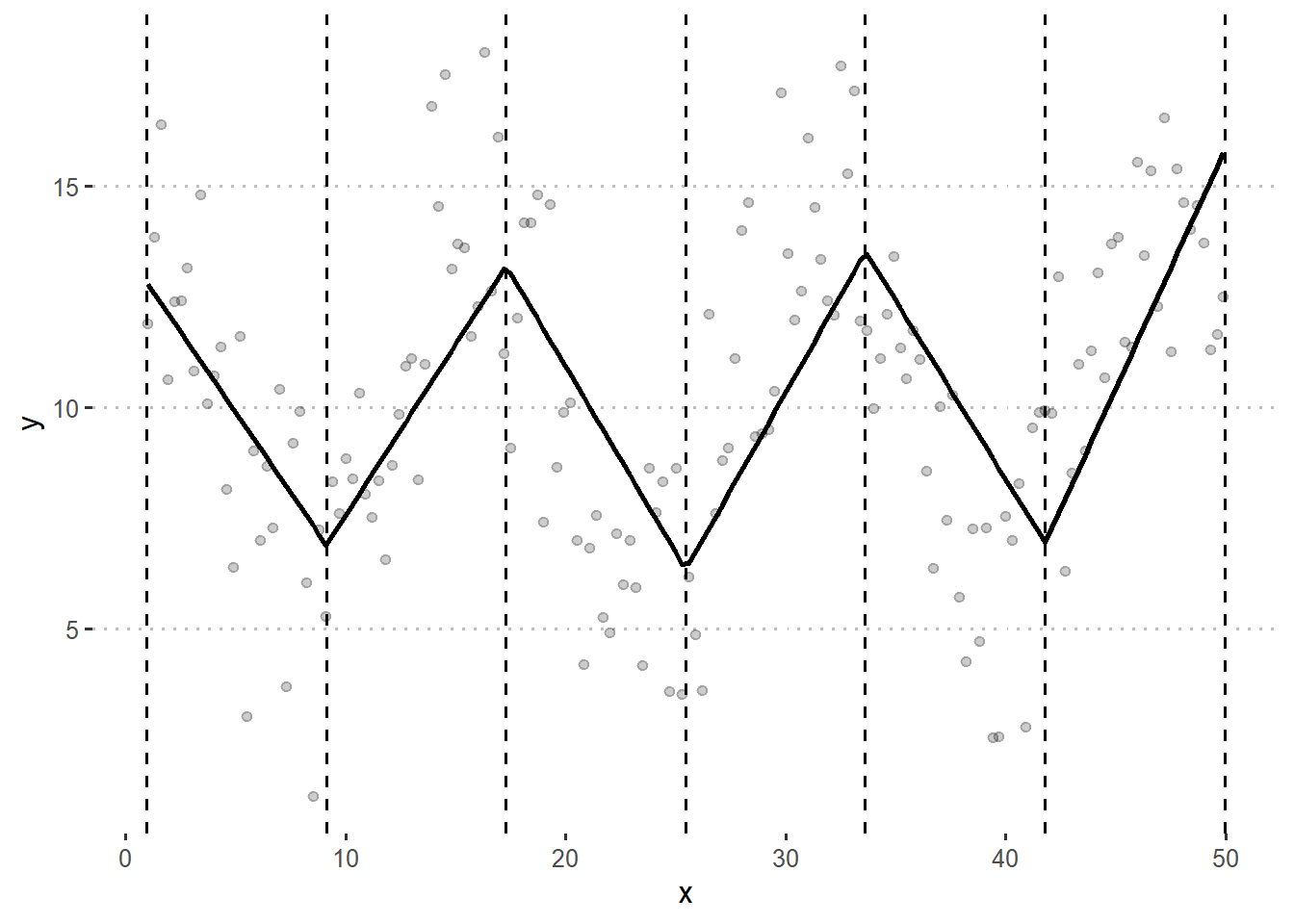
Now, the straight lines might not be the best way to represent the relationship between x and y, not even within each region in x. Now, with \(m=2\) we will have piecewise polynomic regression.
bspline <- gam(y ~ s(x, bs = "bs", m = 2, k=7), data = df)
df$Bspline_m3 <- bspline$fitted.values

knots <- data.frame(knots = bspline$smooth[[1]]$knots[-c(1,2,9,10)])

df %>%
  ggplot(aes(x, y))+
  geom_point(alpha= .2)+
  geom_vline(aes(xintercept = knots), data = knots, linetype =2)+
  geom_line(aes(y = Bspline), size = 1, color = "grey45")+
  geom_line(aes(y = Bspline_m3), size = 1)+
  theme_pubclean()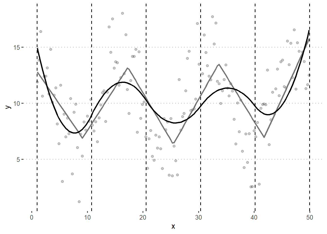
Many questions may arise from looking at this:
- What is the best \(k\)?
- Does a piecewise polynomial really lead to the best results?
16.4.2 Penalized splines
low rank smoothers using a B-spline basis
\(\kappa_1, \kappa_2, \dots, \kappa_K\) are the knots,
\(b_1, b_2, \dots, b_K\) are the spline coefficients.
bspline <- gam(y ~ s(x, bs = "bs", m = 2), data = df)
pspline <- gam(y ~ s(x, bs = "ps", m = 2), data = df)
df$Bspline <- bspline$fitted.values
df$Pspline <- pspline$fitted.values

df <- df %>% pivot_longer(c(Bspline,Pspline), names_to = "spline", values_to = "fitted")

knots <- data.frame(knots = bspline$smooth[[1]]$knots[-c(1, 2,12, 13)])

df %>%
  ggplot(aes(x, y))+
  geom_point(alpha= .2)+
  geom_vline(aes(xintercept = knots), data = knots, linetype =2)+
  geom_line(aes(y = fitted, group = spline, color = spline), size = 1.5)+
  theme_pubclean()+
  labs(color = "Smoothing basis")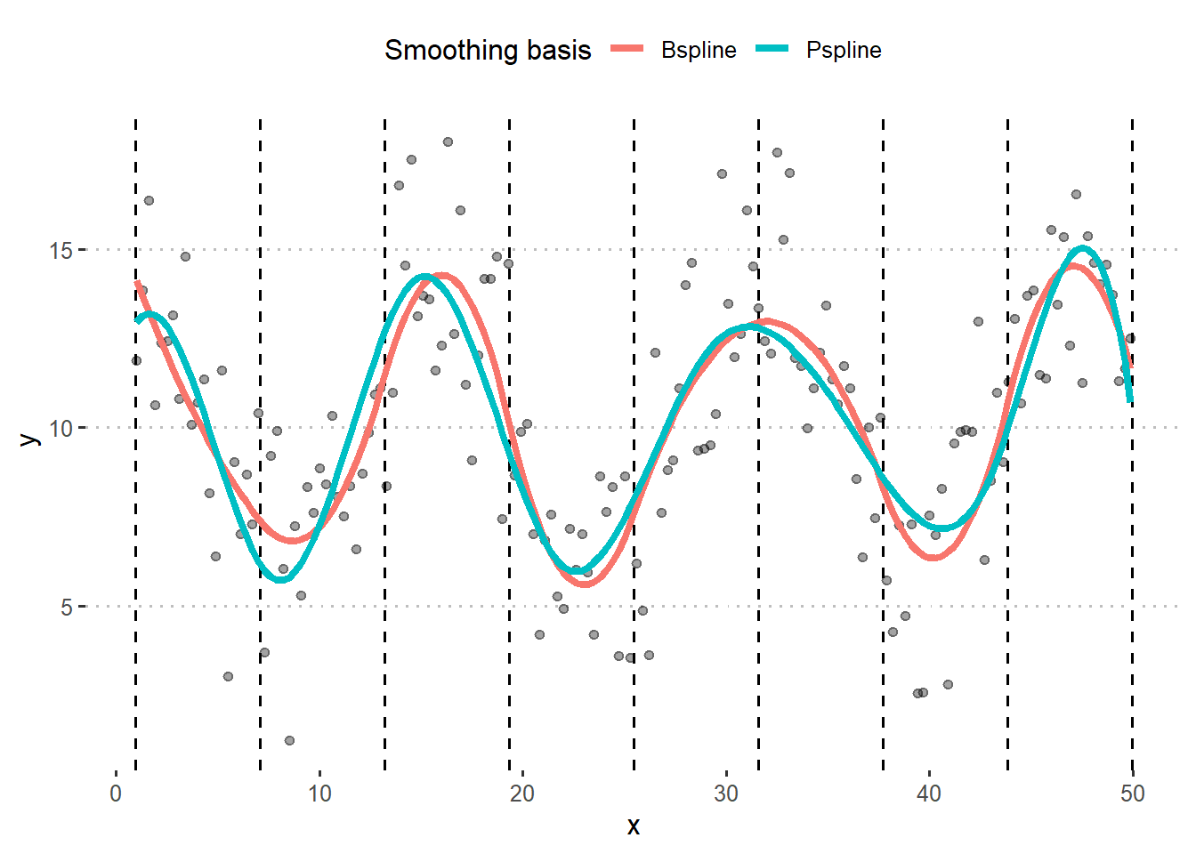
16.5 Final comments
- Generalized additive models
- Choosing parametric vs. semi-parametric
- Choosing types of splines
- Model selection
- G-side vs. R-side discussion
How to apply this in the spatial model from before:
16.6 Resources
- Wood, S.N. (2017). Generalized Additive Models. Chapman and Hall/CRC. [link]
- Ruppert, D. (2004). Nonparametric Regression and Splines. In: Statistics and Finance. Springer Texts in Statistics. Springer, New York, NY. https://doi.org/10.1007/978-1-4419-6876-0_13