Day 7 Generalized Linear Mixed Models
September 17th
7.1 Announcements
- Assignment 2 grades are posted
- Assignment 3 due on Sunday
- This blog post on “bad science”
7.2 Review about the (general) linear mixed model
One of the most common notations is the model equation form:
\[y_{ij} = \mu + T_i + \varepsilon_{ij} , \\ \varepsilon_{ij}\sim N(0, \sigma^2),\] which is very much restrictive.
7.3 Generalized linear mixed models
Now, if we relax the assumption of the normal distributions, there are several other probability distributions that could describe how the data are generated. GLMMs are linear models for variables from any distribution from the exponential family.
Exponential family: pdf can be written as \[f(y\vert \theta) = \exp \begin{bmatrix} \frac{y\theta- b(\theta)}{a(\theta)} + c(y, \phi) \end{bmatrix} ,\] where \(y\) is the random variable (e.g., the response), \(\theta\) is a canonical parameter (related to the mean) and \(\phi\) is a scale parameter (related to the dispersion).
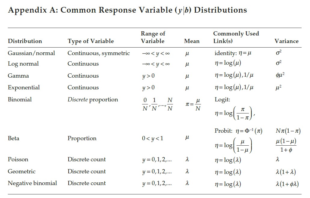
Figure 7.1: Common variable distributions. Page 60 in Stroup et al. (2024)
7.3.1 Three steps to modeling data
- Define the linear predictor \(\boldsymbol\eta = \mathbf{X}\boldsymbol{\beta} + \mathbf{Z}\mathbf{u}\),
- Define the probability distribution for the data, \(\mathbf{y}|\mathbf{u}\),
- Define the link function \(g(\cdot)\), \(\boldsymbol\eta = g(\mathbf{y}|\mathbf{u})\).
7.3.2 Implications for model fitting
- Least Squares Estimator is no longer Maximum Likelihood Estimator
- Variance is no longer \(\hat\sigma^2 = \frac{SSE}{df_e}\)
- The whole concept of degrees of freedom is more diffuse
- ANOVA shells are still useful to analyze designs are number of independent, true, replicates
- The \(Var(\mathbf{y}|\mathbf{u})\) may be specified, but not specify the full likelihood (check out the properties above)
- Quasi-likelihood for modeling overdispersion or repeated measures in GLMMs:
- \(E(\mathbf{y} \vert \mathbf{b}) = \boldsymbol{\mu}\vert \mathbf{b}\)
- \(Var(\mathbf{y} \vert \mathbf{b}) = \mathbf{V}_{\mu}^{1/2}\mathbf{A}\mathbf{V}_{\mu}^{1/2}\)