Day 26 Planning designed experiments

26.1 Announcements

Project deadlines:
- December 12th: give your presentation by this date (it can be earlier than this also). You will need to schedule a 30min meeting with me.
- December 19th: submit your final project and tutorial on canvas, including both your classmate’s and my feedback.

26.2 Designed experiments

On the importace of designed experiments
Defining the data generating process
Statistical power
Precision of parameters

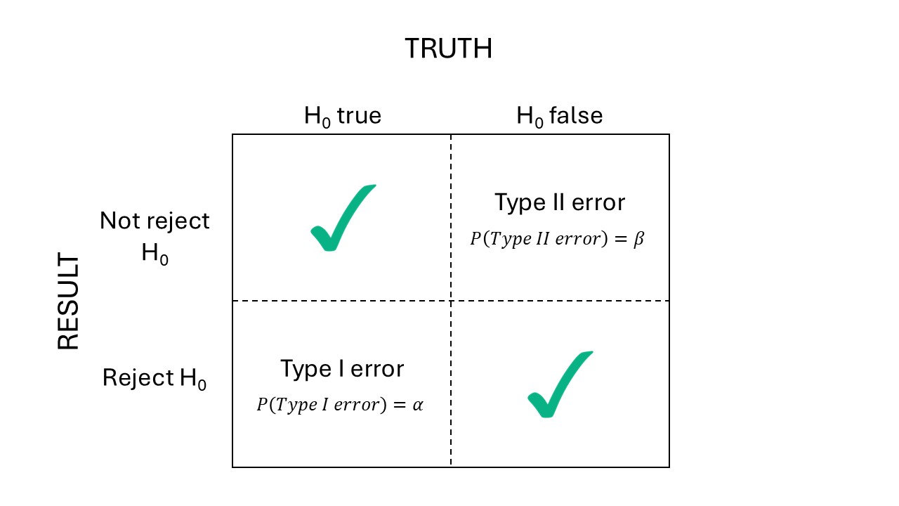
Figure 26.1: Types of errors.

26.2.0.1 Analytical solutions

We know Power is

\[Power = P(F>F_{c} \vert F \sim F(df_1, df_2, \phi)),\]

where:

\(F\) is the F test statistics,
\(F_c\) is the critical test F,
\(df_1\) are the degrees of freedom of the numerator,
\(df_2\) are the degrees of freedom of the denominator,
\(\phi\) is the noncentrality parameter.

Note that \(F\) depends on \(\sigma^2_\varepsilon\), and \(F_c\) depends on \(\alpha\).

Suppose we are trying to compare designs to find differences main effects and interactions of a \(3 \times 2\) factorial treatment structure. Suppose we have:

Treatment A: 3 levels,
Treatment B: 2 levels.

Typically, we would find means around \(10\) units, and \(\sigma^2 \approx 1\).

library(nlme)

This is how a dataframe coudl look like:

n_reps <- 3
data <- 
  purrr::map_dfr(
    seq_len(n_reps),
    ~expand.grid(tA = factor(1:3),
                tB = factor(1:2)) |>
      mutate(mu = c(10,12,12,10,10,12))) |> 
  mutate(rep = rep(1:n_reps, each = 6))
head(data)

##   tA tB mu rep
## 1  1  1 10   1
## 2  2  1 12   1
## 3  3  1 12   1
## 4  1  2 10   1
## 5  2  2 10   1
## 6  3  2 12   1

# Also:

sigma2_e <- 1
sigma2_block <- .8
sigma2_wp <- .2

How do different designs compare?

# create an RCBD model 
m_rcbd <- lme(mu ~ tA * tB, 
         random = list(rep = pdSymm(matrix(sqrt(sigma2_block)), ~ 1, nam = "(Intercept)")), 
         data = data,
         # this won't converge but ask to get an object anyways
         control = lmeControl(
           sigma = sqrt(sigma2_e),
           returnObject = TRUE))


# peek at the variance-covariance matrix 
VarCorr(m_rcbd)

## rep = pdSymm(1) 
##             Variance   StdDev    
## (Intercept) 0.00863157 0.09290624
## Residual    1.00000000 1.00000000

# fix variance components 
m_rcbd$modelStruct$reStruct$rep <-  pdSymm(matrix(sqrt(sigma2_block)), ~ 1, nam = "(Intercept)")

# peek at the variance-covariance matrix again
VarCorr(m_rcbd)

## rep = pdSymm(1) 
##             Variance  StdDev   
## (Intercept) 0.8944272 0.9457416
## Residual    1.0000000 1.0000000

results <-
  emmeans::joint_tests(m_rcbd) |> 
  as.data.frame() |> 
  transmute(source = `model term`, 
            numDF = df1, 
            denDF = df2, 
            F.ratio)

alpha <- 0.05

results |> 
  mutate(ncp = F.ratio* numDF, 
         Fcrit = qf(1-alpha, df1 = numDF, df2 = denDF, ncp = 0),
         Power = 1 - pf(Fcrit, df1 = numDF, df2 = denDF, ncp = ncp))

##   source numDF denDF F.ratio ncp    Fcrit     Power
## 1     tA     2    10       6  12 4.102821 0.7592131
## 3     tB     1    10       2   2 4.964603 0.2490518
## 2  tA:tB     2    10       2   4 4.102821 0.3183418

# create a split-plot model where tA was the whole plot  
m_sp <- lme(mu ~ tA * tB, 
         random = list(rep = pdSymm(matrix(sqrt(sigma2_block)), ~ 1, 
                                    nam = "(Intercept)"), 
                       tA = pdSymm(matrix(sqrt(sigma2_wp)), ~ 1)), 
         data = data,
         # this won't converge but ask to get an object anyways
         control = lmeControl(sigma = sqrt(sigma2_e), 
                              returnObject = TRUE, 
                              maxIter = 0))

# peek at the variance-covariance matrix 
VarCorr(m_sp)

##             Variance   StdDev   
## rep =       pdSymm(1)           
## (Intercept) 0.01216669 0.1103027
## tA =        pdSymm(1)           
## (Intercept) 0.03296807 0.1815711
## Residual    1.00000000 1.0000000

# fix variance components 
m_sp$modelStruct$reStruct$rep <-  pdSymm(matrix(sqrt(sigma2_block)), ~ 1, nam = "(Intercept)")
m_sp$modelStruct$reStruct$tA <-  pdSymm(matrix(sqrt(sigma2_wp)), ~ 1, nam = "(Intercept)")

# peek at the variance-covariance matrix again
VarCorr(m_sp)

##             Variance  StdDev   
## rep =       pdSymm(1)          
## (Intercept) 0.8944272 0.9457416
## tA =        pdSymm(1)          
## (Intercept) 0.4472136 0.6687403
## Residual    1.0000000 1.0000000

results <-
  emmeans::joint_tests(m_sp) |> 
  as.data.frame() |> 
  transmute(source = `model term`, 
            numDF = df1, 
            denDF = df2, 
            F.ratio)

alpha <- 0.05

results |> 
  mutate(ncp = F.ratio* numDF, 
         Fcrit = qf(1-alpha, df1 = numDF, df2 = denDF, ncp = 0),
         Power = 1 - pf(Fcrit, df1 = numDF, df2 = denDF, ncp = ncp))

##   source numDF denDF F.ratio    ncp    Fcrit     Power
## 1     tA     2     4   5.629 11.258 6.944272 0.5146767
## 3     tB     1     6   2.000  2.000 5.987378 0.2231880
## 2  tA:tB     2     6   2.000  4.000 5.143253 0.2682179

26.2.1 Precision analysis

Power analysis versus precision analyses (the focus on p-values)
ASA’s statement on p-values
Scientists rise up against statistical significance
- Discussion
- Counterargument: In defense of p-values
Gelman “Let us have the serenity to embrace the variation that we cannot reduce, the courage to reduce the variation we cannot embrace, and the wisdom to distinguish one from the other.” [see talk]

res <- as.data.frame(emmeans::emmeans(m_rcbd, ~ tA, contr = list(c(1, -1, 0)))$contrasts)

## NOTE: Results may be misleading due to involvement in interactions

res$SE*(qt(p = .975, df = res$df) - qt(p = .025, df = res$df))

## [1] 2.572833

res <- as.data.frame(emmeans::emmeans(m_sp, ~ tA, contr = list(c(1, -1, 0)))$contrasts)

## NOTE: Results may be misleading due to involvement in interactions

res$SE*(qt(p = .975, df = res$df) - qt(p = .025, df = res$df))

## [1] 3.30997

26.3 Bayesian analysis of designed experiments

Bayes theorem:

\[[\boldsymbol{\theta} \vert \mathbf{y}] = \frac{[\mathbf{y} \vert \boldsymbol{\theta}] [\boldsymbol{\theta}] }{ [\mathbf{y}]}, \]

where:

\([\boldsymbol{\theta} \vert \mathbf{y}]\) is the posterior distribution,
\([\mathbf{y} \vert \boldsymbol{\theta}]\) is the likelihood,
\([\boldsymbol{\theta}]\) is the prior,
\([\mathbf{y}]\) is the data.

Note that whatever is defined in \([\cdot]\), it’s information.

26.4 Applied example

Suppose we designed an experiment with the rationale outlined above. What if the model doesn’t converge?

About dropping effects from the model
Bayesian solutions

library(glmmTMB)
library(ggpubr)

dat <- readxl::read_xlsx("../../data_confid/Behavior_Counts.xlsx")

# viz
dat |> 
  ggplot(aes(timepoint, behavior_count))+
  geom_line(aes(group = calfID, 
                color = breed))+
  geom_point(aes(group = breed, 
                 fill = breed),
             shape =21, size= 2.5)+
  facet_wrap(~trt)+
  scico::scale_fill_scico_d()+
  scico::scale_color_scico_d()+
  theme_pubclean()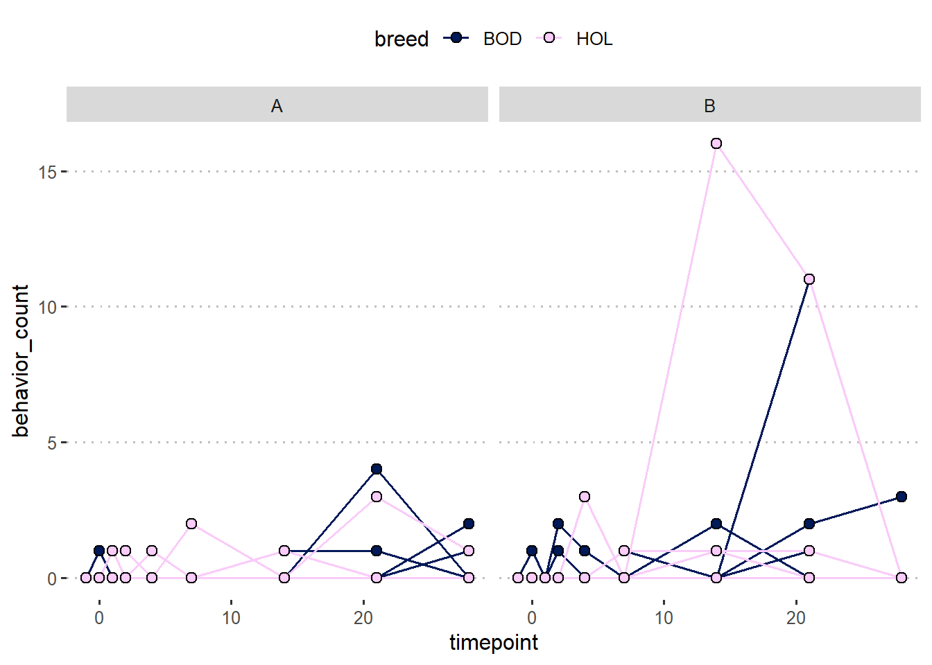

m2 <- glmmTMB(behavior_count ~ timepoint * trt * breed +
                toep(timepoint + 0 | calfID),
              ziformula = ~1,
              family = poisson(link = "log"),
              data = dat |> mutate(timepoint_f=as.factor(timepoint)))

What to do?

Link to R code

STAT 870 - Analysis of Messy Data