Day 23 Integrating multi-environment trials with weather data
23.1 Announcements
- Office hours tomorrow have moved to 11.30-12.30.
- Project deadlines:
- November 28th: send your project to your classmate(s) for peer review.
- December 5th: return your peer review to your classmate(s).
- December 12th: give your presentation by this date (it can be earlier than this also). You will need to schedule a 30min meeting with me.
- December 19th: submit your final project and tutorial on canvas, including both your classmate’s and my feedback.
23.2 Opportunistic use of multi-environment trials
- Objective of an experiment
- Review of designed experiments
- Bias-Variance tradeoff
- Power in these analyses
##
## Call:
## lm(formula = yield ~ srad_total + ppt_total + factor(hyb), data = d)
##
## Residuals:
##     Min      1Q  Median      3Q     Max
## -2.1482 -0.4294  0.0000  0.4380  1.8558
##
## Coefficients:
##                Estimate Std. Error t value Pr(>|t|)
## (Intercept)   -60.69421    5.01929 -12.092  < 2e-16 ***
## srad_total     29.73582    2.01150  14.783  < 2e-16 ***
## ppt_total       0.78573    0.11883   6.612 3.70e-10 ***
## factor(hyb)2    4.48472    0.75051   5.976 1.10e-08 ***
## factor(hyb)3    1.52404    0.65572   2.324 0.021166 *
## factor(hyb)4    0.64319    0.75051   0.857 0.392520
## factor(hyb)5   -2.87003    0.64272  -4.465 1.36e-05 ***
## factor(hyb)6   -1.15626    0.64272  -1.799 0.073596 .
## factor(hyb)7    0.96009    0.64272   1.494 0.136878
## factor(hyb)8   -2.78208    0.64272  -4.329 2.42e-05 ***
## factor(hyb)9  -10.40201    0.90894 -11.444  < 2e-16 ***
## factor(hyb)10  -1.13644    0.92639  -1.227 0.221430
## factor(hyb)11  -2.41343    0.68319  -3.533 0.000516 ***
## factor(hyb)12  -4.23456    0.93800  -4.514 1.11e-05 ***
## factor(hyb)13   6.11476    0.63617   9.612  < 2e-16 ***
## factor(hyb)14  -2.50853    0.96169  -2.608 0.009815 **
## factor(hyb)15  -4.25297    0.58881  -7.223 1.18e-11 ***
## factor(hyb)16  -7.72464    0.96768  -7.983 1.30e-13 ***
## factor(hyb)17   3.78123    0.60713   6.228 2.94e-09 ***
## factor(hyb)18   5.02229    0.75550   6.648 3.04e-10 ***
## factor(hyb)19  -2.23794    0.78424  -2.854 0.004799 **
## factor(hyb)20   3.02746    0.71538   4.232 3.59e-05 ***
## factor(hyb)21  -4.70163    0.72448  -6.490 7.22e-10 ***
## factor(hyb)22  -1.74531    0.64657  -2.699 0.007571 **
## factor(hyb)23   1.44812    0.57856   2.503 0.013154 *
## factor(hyb)24   4.72568    0.98698   4.788 3.37e-06 ***
## factor(hyb)25   4.51208    0.67110   6.723 2.00e-10 ***
## factor(hyb)26  -6.35203    0.64657  -9.824  < 2e-16 ***
## factor(hyb)27   2.85905    0.68246   4.189 4.27e-05 ***
## factor(hyb)28   3.69420    0.93439   3.954 0.000108 ***
## factor(hyb)29   4.46544    0.81506   5.479 1.34e-07 ***
## factor(hyb)30  -8.46296    0.75320 -11.236  < 2e-16 ***
## factor(hyb)31   3.31140    0.75051   4.412 1.71e-05 ***
## factor(hyb)32  -4.10483    0.64657  -6.349 1.55e-09 ***
## factor(hyb)33   2.71563    0.78424   3.463 0.000660 ***
## factor(hyb)34   9.05725    0.96889   9.348  < 2e-16 ***
## factor(hyb)35   2.63563    0.71858   3.668 0.000317 ***
## factor(hyb)36   9.73918    0.92639  10.513  < 2e-16 ***
## factor(hyb)37  -2.28390    0.75550  -3.023 0.002846 **
## factor(hyb)38   1.27240    0.66491   1.914 0.057161 .
## factor(hyb)39  -2.61287    0.71683  -3.645 0.000345 ***
## factor(hyb)40   3.51171    0.96889   3.624 0.000371 ***
## factor(hyb)41  -3.98966    0.64272  -6.207 3.28e-09 ***
## factor(hyb)42  -0.42630    0.67561  -0.631 0.528805
## factor(hyb)43   0.48600    0.61137   0.795 0.427644
## factor(hyb)44  -0.58237    0.68137  -0.855 0.393787
## factor(hyb)45   4.15067    0.71683   5.790 2.85e-08 ***
## factor(hyb)46  -3.64700    0.81667  -4.466 1.36e-05 ***
## factor(hyb)47  -0.72016    0.64548  -1.116 0.265957
## factor(hyb)48  -0.84831    0.67275  -1.261 0.208866
## factor(hyb)49  -4.22068    0.67296  -6.272 2.33e-09 ***
## factor(hyb)50  -1.12484    0.60208  -1.868 0.063258 .
## factor(hyb)51  -2.69567    0.63375  -4.254 3.29e-05 ***
## factor(hyb)52  -1.93346    0.55661  -3.474 0.000635 ***
## factor(hyb)53   0.02128    0.64272   0.033 0.973619
## factor(hyb)54   5.52610    0.71858   7.690 7.57e-13 ***
## factor(hyb)55 -10.20572    0.64657 -15.784  < 2e-16 ***
## factor(hyb)56   1.75090    0.75550   2.318 0.021533 *
## factor(hyb)57  -1.29931    0.75500  -1.721 0.086879 .
## factor(hyb)58   1.65498    0.62242   2.659 0.008504 **
## factor(hyb)59   2.70007    0.64657   4.176 4.51e-05 ***
## factor(hyb)60  -4.65485    0.64657  -7.199 1.35e-11 ***
## factor(hyb)61  -2.50210    0.67296  -3.718 0.000264 ***
## factor(hyb)62  -3.38133    0.61137  -5.531 1.04e-07 ***
## factor(hyb)63  -0.65019    0.71538  -0.909 0.364565
## factor(hyb)64   1.03107    0.59772   1.725 0.086144 .
## factor(hyb)65   5.33124    0.93840   5.681 4.93e-08 ***
## factor(hyb)66  -5.10546    0.62532  -8.165 4.28e-14 ***
## factor(hyb)67   5.22070    0.93840   5.563 8.85e-08 ***
## factor(hyb)68   0.94839    0.62532   1.517 0.131007
## factor(hyb)69   2.17529    0.63509   3.425 0.000752 ***
## factor(hyb)70  -0.96006    0.73261  -1.310 0.191615
## factor(hyb)71   1.94152    0.81667   2.377 0.018424 *
## factor(hyb)72  -0.18008    0.60062  -0.300 0.764639
## factor(hyb)73  -1.91320    0.54730  -3.496 0.000588 ***
## factor(hyb)74  -2.21349    0.52530  -4.214 3.87e-05 ***
## factor(hyb)75  -6.69256    0.96768  -6.916 6.80e-11 ***
## factor(hyb)76  -0.44575    0.93800  -0.475 0.635175
## factor(hyb)77   3.10083    0.73261   4.233 3.59e-05 ***
## factor(hyb)78  -1.00358    0.67617  -1.484 0.139399
## factor(hyb)79   4.84662    0.67617   7.168 1.62e-11 ***
## factor(hyb)80  -3.09158    0.65462  -4.723 4.50e-06 ***
## factor(hyb)81   1.34925    0.55397   2.436 0.015785 *
## factor(hyb)82  -0.74675    0.81667  -0.914 0.361666
## factor(hyb)83   3.46643    0.62903   5.511 1.15e-07 ***
## factor(hyb)84  -4.02740    0.74602  -5.398 1.98e-07 ***
## factor(hyb)85  -1.88953    0.95563  -1.977 0.049450 *
## factor(hyb)86  -2.39751    0.57486  -4.171 4.61e-05 ***
## factor(hyb)87   0.62381    0.71538   0.872 0.384307
## factor(hyb)88  -0.37733    0.73261  -0.515 0.607117
## factor(hyb)89  -2.43654    0.64272  -3.791 0.000201 ***
## factor(hyb)90  -2.70215    0.64272  -4.204 4.02e-05 ***
## factor(hyb)91  -4.50509    0.64272  -7.009 4.01e-11 ***
## factor(hyb)92  -7.89450    0.95563  -8.261 2.37e-14 ***
## ---
## Signif. codes:  0 '***' 0.001 '**' 0.01 '*' 0.05 '.' 0.1 ' ' 1
##
## Residual standard error: 0.7872 on 191 degrees of freedom
## Multiple R-squared:  0.9653, Adjusted R-squared:  0.9484
## F-statistic: 57.12 on 93 and 191 DF,  p-value: < 2.2e-16
m2 <- lmer(yield ~ srad_total + ppt_total + factor(hyb) +
(1|sy),
data = d)
DHARMa::simulateResiduals(m2, plot = T)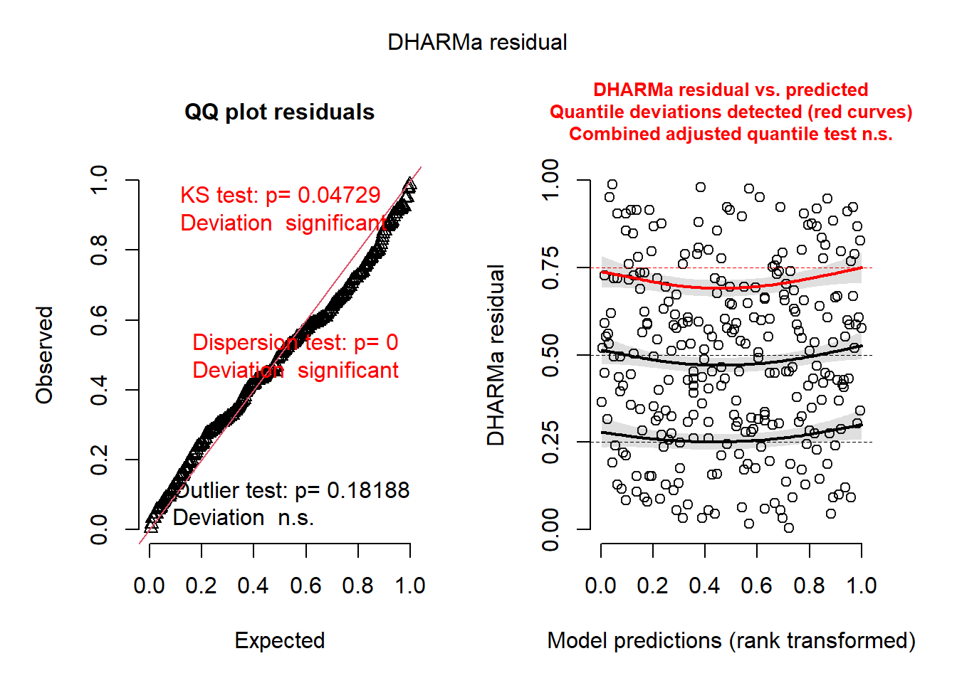
## Object of Class DHARMa with simulated residuals based on 250 simulations with refit = FALSE . See ?DHARMa::simulateResiduals for help.
##
## Scaled residual values: 0.532 0.528 0.552 0.448 0.196 0.604 0.128 0.34 0.696 0.296 0.592 0.368 0.452 0.704 0.136 0.276 0.512 0.324 0.364 0.144 ...## Linear mixed model fit by REML ['lmerMod']
## Formula: yield ~ srad_total + ppt_total + factor(hyb) + (1 | sy)
## Data: d
##
## REML criterion at convergence: 537.1
##
## Scaled residuals:
## Min 1Q Median 3Q Max
## -2.6232 -0.5357 0.0000 0.5625 2.2864
##
## Random effects:
## Groups Name Variance Std.Dev.
## sy (Intercept) 0.0912 0.3020
## Residual 0.5826 0.7633
## Number of obs: 285, groups: sy, 16
##
## Fixed effects:
## Estimate Std. Error t value
## (Intercept) -58.38763 7.17973 -8.132
## srad_total 28.89046 2.87023 10.066
## ppt_total 0.78771 0.16758 4.700
## factor(hyb)2 4.34381 0.80391 5.403
## factor(hyb)3 1.30026 0.70485 1.845
## factor(hyb)4 0.50228 0.80391 0.625
## factor(hyb)5 -2.87003 0.62319 -4.605
## factor(hyb)6 -1.15626 0.62319 -1.855
## factor(hyb)7 0.96009 0.62319 1.541
## factor(hyb)8 -2.78208 0.62319 -4.464
## factor(hyb)9 -10.40201 0.88133 -11.803
## factor(hyb)10 -1.38617 0.96221 -1.441
## factor(hyb)11 -3.01797 0.74751 -4.037
## factor(hyb)12 -4.83909 0.97321 -4.972
## factor(hyb)13 5.63725 0.69455 8.116
## factor(hyb)14 -2.81518 0.99068 -2.842
## factor(hyb)15 -4.62097 0.65763 -7.027
## factor(hyb)16 -8.02757 1.02003 -7.870
## factor(hyb)17 3.38958 0.67239 5.041
## factor(hyb)18 4.52533 0.79784 5.672
## factor(hyb)19 -2.54459 0.83076 -3.063
## factor(hyb)20 2.72081 0.77011 3.533
## factor(hyb)21 -4.77889 0.78588 -6.081
## factor(hyb)22 -2.17785 0.68954 -3.158
## factor(hyb)23 1.29865 0.64397 2.017
## factor(hyb)24 4.55199 0.99712 4.565
## factor(hyb)25 4.30745 0.72587 5.934
## factor(hyb)26 -6.78457 0.68954 -9.839
## factor(hyb)27 2.61889 0.71997 3.638
## factor(hyb)28 3.55329 0.96827 3.670
## factor(hyb)29 4.29175 0.83843 5.119
## factor(hyb)30 -8.66084 0.80181 -10.802
## factor(hyb)31 3.17049 0.80391 3.944
## factor(hyb)32 -4.53737 0.68954 -6.580
## factor(hyb)33 2.40898 0.83076 2.900
## factor(hyb)34 8.50653 1.01009 8.422
## factor(hyb)35 2.63563 0.69675 3.783
## factor(hyb)36 9.48946 0.96221 9.862
## factor(hyb)37 -2.78086 0.79784 -3.486
## factor(hyb)38 0.95652 0.71715 1.334
## factor(hyb)39 -2.88135 0.75661 -3.808
## factor(hyb)40 2.96099 1.01009 2.931
## factor(hyb)41 -3.98966 0.62319 -6.402
## factor(hyb)42 -0.74645 0.72544 -1.029
## factor(hyb)43 0.43157 0.67208 0.642
## factor(hyb)44 -0.85947 0.72467 -1.186
## factor(hyb)45 3.88219 0.75661 5.131
## factor(hyb)46 -3.85761 0.86285 -4.471
## factor(hyb)47 -0.80340 0.63635 -1.263
## factor(hyb)48 -1.20209 0.71876 -1.672
## factor(hyb)49 -4.62825 0.72615 -6.374
## factor(hyb)50 -1.37456 0.67809 -2.027
## factor(hyb)51 -3.12280 0.69476 -4.495
## factor(hyb)52 -1.93346 0.53970 -3.582
## factor(hyb)53 0.02128 0.62319 0.034
## factor(hyb)54 5.52610 0.69675 7.931
## factor(hyb)55 -10.63825 0.68954 -15.428
## factor(hyb)56 1.25394 0.79784 1.572
## factor(hyb)57 -1.90384 0.80985 -2.351
## factor(hyb)58 1.36786 0.67695 2.021
## factor(hyb)59 2.26754 0.68954 3.288
## factor(hyb)60 -5.08738 0.68954 -7.378
## factor(hyb)61 -2.90967 0.72615 -4.007
## factor(hyb)62 -3.43575 0.67208 -5.112
## factor(hyb)63 -0.95683 0.77011 -1.242
## factor(hyb)64 0.85349 0.64680 1.320
## factor(hyb)65 4.83428 0.96323 5.019
## factor(hyb)66 -5.38115 0.67549 -7.966
## factor(hyb)67 4.72374 0.96323 4.904
## factor(hyb)68 0.67270 0.67549 0.996
## factor(hyb)69 1.85635 0.69229 2.681
## factor(hyb)70 -0.99164 0.78813 -1.258
## factor(hyb)71 1.73092 0.86285 2.006
## factor(hyb)72 -0.65737 0.66100 -0.995
## factor(hyb)73 -2.14247 0.55117 -3.887
## factor(hyb)74 -2.35766 0.51826 -4.549
## factor(hyb)75 -6.99549 1.02003 -6.858
## factor(hyb)76 -1.05028 0.97321 -1.079
## factor(hyb)77 3.06925 0.78813 3.894
## factor(hyb)78 -1.38186 0.72665 -1.902
## factor(hyb)79 4.46835 0.72665 6.149
## factor(hyb)80 -3.46014 0.69722 -4.963
## factor(hyb)81 1.06771 0.61617 1.733
## factor(hyb)82 -0.95736 0.86285 -1.110
## factor(hyb)83 3.20216 0.68216 4.694
## factor(hyb)84 -4.45452 0.79267 -5.620
## factor(hyb)85 -2.19680 0.99851 -2.200
## factor(hyb)86 -2.39751 0.55740 -4.301
## factor(hyb)87 0.31716 0.77011 0.412
## factor(hyb)88 -0.40892 0.78813 -0.519
## factor(hyb)89 -2.43654 0.62319 -3.910
## factor(hyb)90 -2.70215 0.62319 -4.336
## factor(hyb)91 -4.50509 0.62319 -7.229
## factor(hyb)92 -8.20178 0.99851 -8.214##
## Correlation matrix not shown by default, as p = 94 > 12.
## Use print(x, correlation=TRUE) or
## vcov(x) if you need it23.3 Power analyses
Let’s first review the different types of errors:
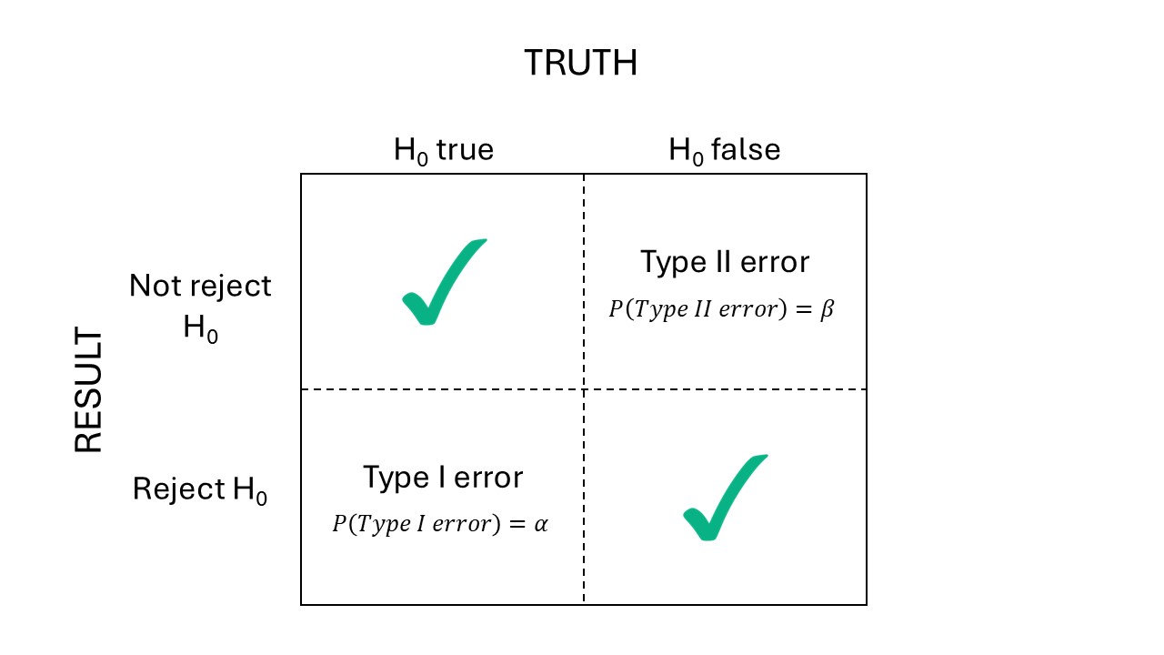
Figure 23.1: Types of error
We normally control \(\alpha\), the probability of doing an error of type I. TO describe our experiment’s ability to detect scientific discoveries, we consider power: the \(P(\text{reject } H_0 | H_0 \text{ false}) = 1- \beta\). Very often, research teams consider 0.8 power as the minimum for an experiment.
23.3.1 Power calculations
23.3.1.1 Analytical solutions
t-test
- Used to evaluate differences between treatment effects or means.
- Example testing against zero: \(t^{\star} = \frac{\hat\theta - 0}{s.e.(\hat\theta)} = \frac{\hat\theta - 0}{s.d.(\hat\theta)/\sqrt{n}}\)
- Note the sensibility to sample size.
- Also, remember the \(s.e.(\hat\theta)\) may differ depending on the design:
- \(s.e.(\hat\theta)\) may depend on \(\sigma^2_\varepsilon\) only (e.g., CRD, RCBD, mean comparisons between treatment levels of the treatment at the split-plot level), \(s.e.(\hat\theta) = \sqrt{\frac{2 \sigma^2_{\varepsilon}}{r t}}\).
- \(s.e.(\hat\theta)\) may depend on \(\sigma^2_\varepsilon\) and \(\sigma^2_{whole \ plot}\) (e.g., mean comparisons between treatment levels of the treatment at the whole-plot level), \(s.e.(\hat\theta) = \sqrt{\frac{2 (\sigma^2_{\varepsilon} + b \cdot \sigma^2_w)}{b \cdot r}}\)
To detect a difference \(\delta\): \[n = \frac{2\hat{\sigma}^2}{\delta^2}[t_{\alpha/2, \nu} + t_{\beta, \nu}]^2,\] where:
- \(n\) is the sample size,
- \(\hat\sigma^2\) is the estimate of \(\sigma^2\) based on \(\nu\) degrees of freedom,
- \(\alpha\) is the type I error rate,
- \(\beta\) is the type II error rate,
- And note that: \(Var(\delta)=2\sigma^2/n\).
23.3.1.2 Simulation solutions
Below is a simulation comparing 3 different scenarios of multi-environment trials with different number of environments tested. We assume that, within each environment, the trial is an RCBD with three repetitions. [Context: this is perhaps the most common design in agronomy.]
We assume the following data generating process: \[y_{ijk} = \mu_i + b_{j(k)} + u_k +\varepsilon_{ijk}, \\ b_{j(k)} \sim N(0, \sigma_{b}^2), \\ u_k \sim N(0, \sigma_{u}^2), \\ \varepsilon_{ijk} \sim N(0, \sigma_{\varepsilon}^2),\] where:
- \(\mu_i\) is the treatment mean for the \(i\)th treatment (\(i = 1,2, ..., 30\)),
- \(b_{j(k)}\) is the effect of the \(j\)th block in the \(k\)th environment (\(j = 1,2,3\)),
- \(u_k\) is the effect of the \(k\)th environment (\(k = 1,2,..., E\)), and
- \(\varepsilon_{ijk}\) is the residual for the observation corresponding to the \(i\)th treatment, \(j\)th block in the \(k\)th environment.
For this simulation, we assume that all \(b_{j(k)}\), \(u_k\) and \(\varepsilon_{ijk}\) arise from independent normal distributions, with variances \(\sigma_{b}^2 = 3\), \(\sigma_{u}^2 = 35\), \(\sigma_{\varepsilon}^2 = 10\).
Each simulation consists of 3 steps:
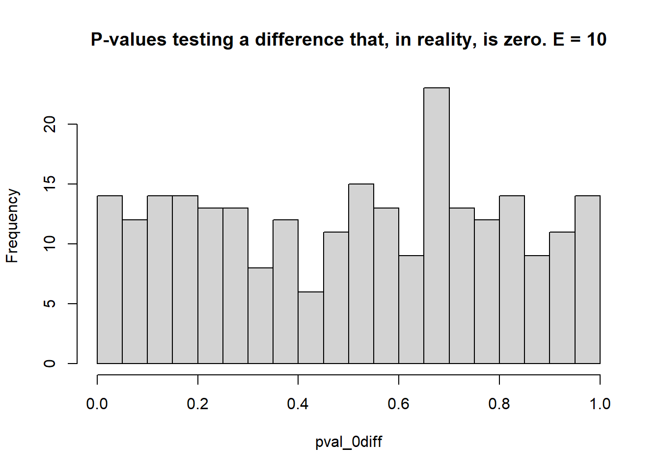
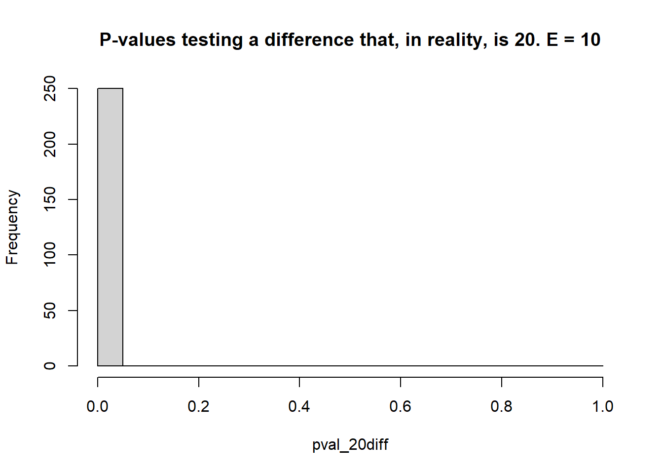
- Set “true” states (i.e., set \(\mu_i\)). We assume the same “ground truth” for all cases. To demonstrate the properties of the designs, we will assume some treatments have no difference (i.e., \(\mu_i = \mu_{i'}\)) and others are different (i.e., \(\mu_i \neq \mu_{i'}\)). Note: this step does not depend on sample size.
- Draw random samples from \(b_{j(k)}\), \(u_k\) and \(\varepsilon_{ijk}\) to simulate observed values \(y_{ijk}\). Note: this step depends on sample size.
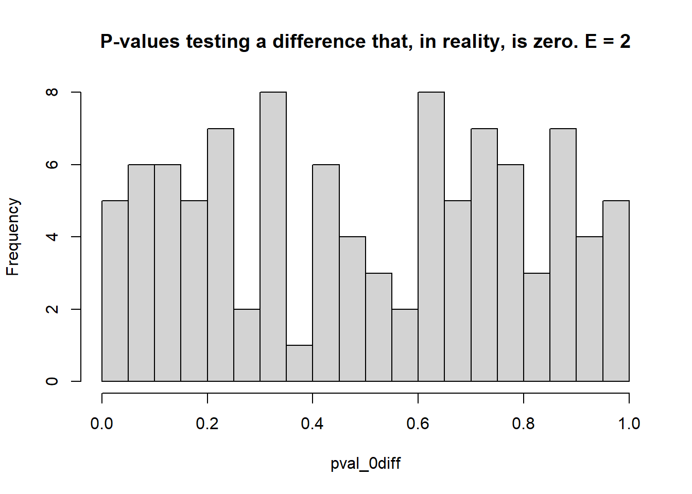
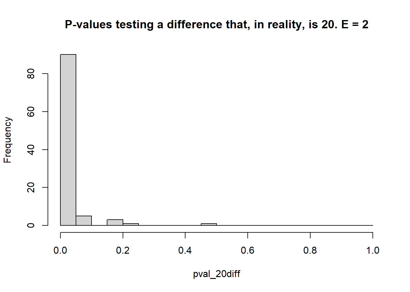
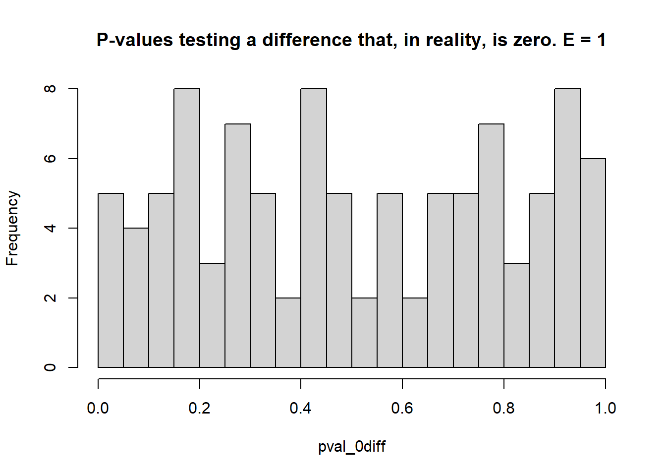
- Estimate the \(\mu_i\)s and test the type I error rate (count of times when \(p<0.05\) when the truth was actually \(\mu_i = \mu_{i'}\) – reject \(H_0\) when it was true), and the statistical power (count of times when \(p<0.05\) when the truth was \(\mu_i \ne \mu_{i'}\) – reject \(H_0\) when it was false).
R packages required for this simulation
library(tidyverse) # data wrangling & data viz
library(lme4) # model fitting
library(emmeans) # marginal means
Simulate 100 hypothetical experiments for 3 scenarios:
- 10 environments, 3 blocks each
Click to show code for the simulation
sigma_env.truth <- 35
sigma_block.truth <- 3
sigma.truth <- 10

trts <- paste("t", 11:40, sep = "")
n_envs <- 10
n_rep <- 3
n_sims <- 250

df_me <- expand.grid(trt = trts,
                     rep = 1:n_rep,
                     environm = paste("e", 11:(10+n_envs), sep = ""))

pval_0diff <- numeric(n_sims)
pval_20diff <- numeric(n_sims)

for (i in 1:n_sims) {
  env_re <- rnorm(n_envs, 0, sigma_env.truth)
  block_re <- rnorm(n_envs*n_rep, 0, sigma_block.truth)

  df_envs <- data.frame(environm = paste("e", 11:(10+n_envs), sep = ""),
                        env_re)
  df_blocks <- expand.grid(environm = paste("e", 11:(10+n_envs), sep = ""),
                           rep = 1:n_rep) %>%
    mutate(block_re = block_re)

  df_me <- df_me %>%
    mutate(mu_t = case_when(trt == "t11" ~ 200,
                            trt == "t12" ~ 200,
                            trt == "t13" ~ 180,
                            .default = 220)) %>%
    left_join(df_envs) %>%
    left_join(df_blocks) %>%
    mutate(e = rnorm(nrow(df_me), 0, sigma.truth),
           y = mu_t + env_re + block_re + e)


  m <- lmer(y ~ trt + (1|environm/rep), data = df_me)
  pval_0diff[i] <- as.data.frame(emmeans(m, ~ trt, contr = list(c(1, -1, rep(0, 28))))$contr)$p.value
  pval_20diff[i] <- as.data.frame(emmeans(m, ~ trt, contr = list(c(1, 0, 0, -1, rep(0, 26))))$contr)$p.value
} 
## [1] 0.056## [1] 1- 2 environments, 3 blocks each
Click to show code for the simulation
sigma_env.truth <- 35
sigma_block.truth <- 3
sigma.truth <- 10

trts <- paste("t", 11:40, sep = "")
n_envs <- 2
n_rep <- 3
n_sims <- 100

df_me <- expand.grid(trt = trts,
                     rep = 1:n_rep,
                     environm = paste("e", 11:(10+n_envs), sep = ""))

pval_0diff <- numeric(n_sims)
pval_20diff <- numeric(n_sims)

set.seed(3)
for (i in 1:n_sims) {
  env_re <- rnorm(n_envs, 0, sigma_env.truth)
  block_re <- rnorm(n_envs*n_rep, 0, sigma_block.truth)

  df_envs <- data.frame(environm = paste("e", 11:(10+n_envs), sep = ""),
                        env_re)
  df_blocks <- expand.grid(environm = paste("e", 11:(10+n_envs), sep = ""),
                           rep = 1:n_rep) %>%
    mutate(block_re = block_re)

  df_me <- df_me %>%
    mutate(mu_t = case_when(trt == "t11" ~ 200,
                            trt == "t12" ~ 200,
                            trt == "t13" ~ 180,
                            .default = 220)) %>%
    left_join(df_envs) %>%
    left_join(df_blocks) %>%
    mutate(e = rnorm(nrow(df_me), 0, sigma.truth),
           y = mu_t + env_re + block_re + e)


  m <- lmer(y ~ trt + (1|environm/rep), data = df_me)
  pval_0diff[i] <- as.data.frame(emmeans(m, ~ trt, contr = list(c(1, -1, rep(0, 28))))$contr)$p.value
  pval_20diff[i] <- as.data.frame(emmeans(m, ~ trt, contr = list(c(1, 0, 0, -1, rep(0, 26))))$contr)$p.value
}
## [1] 0.05## [1] 0.9- 1 environment, 3 blocks each
Click to show code for the simulation
sigma_env.truth <- 35
sigma_block.truth <- 3
sigma.truth <- 10

trts <- paste("t", 11:40, sep = "")
n_envs <- 1
n_rep <- 3
n_sims <- 100

df_me <- expand.grid(trt = trts,
                     rep = 1:n_rep,
                     environm = paste("e", 11:(10+n_envs), sep = ""))

pval_0diff <- numeric(n_sims)
pval_20diff <- numeric(n_sims)

set.seed(3)
for (i in 1:n_sims) {
  env_re <- rnorm(n_envs, 0, sigma_env.truth)
  block_re <- rnorm(n_envs*n_rep, 0, sigma_block.truth)

  df_envs <- data.frame(environm = paste("e", 11:(10+n_envs), sep = ""),
                        env_re)
  df_blocks <- expand.grid(environm = paste("e", 11:(10+n_envs), sep = ""),
                           rep = 1:n_rep) %>%
    mutate(block_re = block_re)

  df_me <- df_me %>%
    mutate(mu_t = case_when(trt == "t11" ~ 200,
                            trt == "t12" ~ 200,
                            trt == "t13" ~ 180,
                            .default = 220)) %>%
    left_join(df_envs) %>%
    left_join(df_blocks) %>%
    mutate(e = rnorm(nrow(df_me), 0, sigma.truth),
           y = mu_t + env_re + block_re + e)


  m <- lmer(y ~ trt + (1|rep), data = df_me)
  pval_0diff[i] <- as.data.frame(emmeans(m, ~ trt, contr = list(c(1, -1, rep(0, 28))))$contr)$p.value
  pval_20diff[i] <- as.data.frame(emmeans(m, ~ trt, contr = list(c(1, 0, 0, -1, rep(0, 26))))$contr)$p.value
}
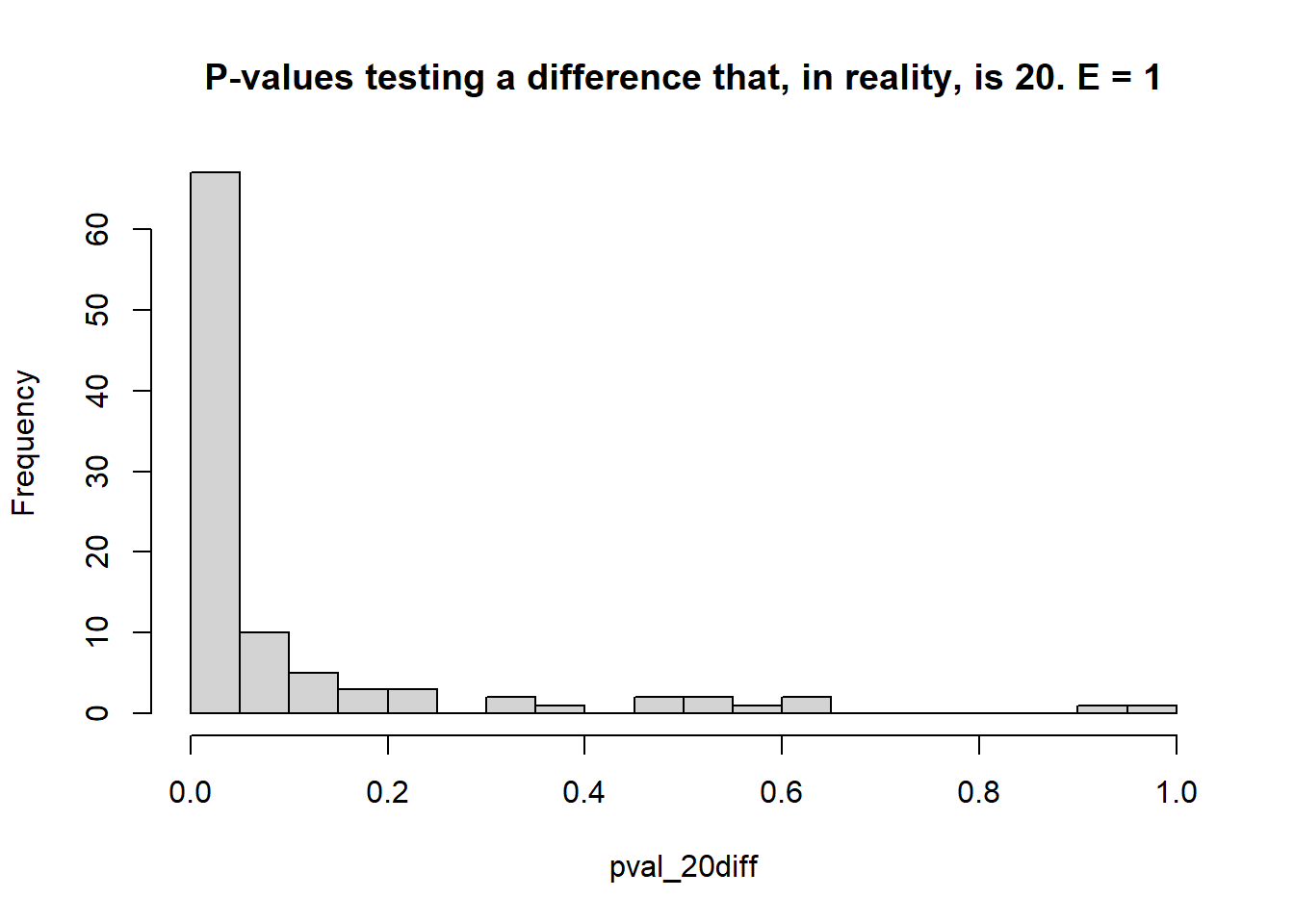
## [1] 0.05## [1] 0.67